
Tutorial to the anomaly vegetation change detection: “AVOCADO”
2025-03-11
Mathieu Decuyper, Roberto O. Chávez, José A. Lastra
Introduction
The “AVOCADO” (Anomaly Vegetation Change Detection) algorithm is a continuous vegetation change detection method that also capture regrowth (Decuyper et al., 2022). It is based on the R package npphen (Chávez et. al., 2023), developed to monitor phenology changes, and adjusted to monitor forest disturbance and regrowth in a semi-automated and continuous way. The algorithm uses all available data and does not require certain pre-processing steps such as removing outliers. The reference vegetation (undisturbed forest in this case) is taken from nearby pixels that are known to be undisturbed during the whole time-series, so there is no need to set aside part of the time-series as an historical baseline. By using the complete time-series in AVOCADO, more robust predictions of vegetation changes can be made while improving our ability to deal with gaps in the data. The algorithm accounts for the natural variability of the annual phenology (using the flexibility of Kernel fitting), which makes it potentially more suitable to monitor areas with strong seasonality (e.g. dry ecosystems) and gradual/small changes (i.e. degradation).
Step 1: Installing the required packages
| library(remotes) install_github('MDecuy/AVOCADO') # Load library library(AVOCADO) |
Please note that an explanation on all parameters of the AVOCADO algorithm can be found in the github documentation and the paper Decuyper et al., 2022.
Within the package you will find several functions:
- The PhenRef2d() function, which is used to create the reference phenology for the reference forest area.
- To explore at pixel level you will need the functions PLUGPhenAnoRFDPLUS() and dist.reg().
- To create a wall-to-wall map as a result you will need the functions PLUGPhenAnoRFDMapPLUS() and dist.reg.map().
Other R-packages that AVOCADO relies on and are required: terra and lubridate.
Some suggested R-packages are npphen and parallel
Important: Please note that for the mapping part you might need quite some computational power (i.e. multi-CPU computer), depending on the size of your study area and the length of the time-series. This does NOT apply for the example area in this tutorial.
Step 2: Downloading the satellite data
Currently there are various satellite sources and ways to download the data such as the Earth Explorer or the Google Earth Engine platform (Gorelick et al., 2017). There is a lot information on how to download various satellite data on the Google Earth Engine Guides platform, but here we provide a small example GEE script for Landsat data.
The first step is to upload the shapefile for your area of interest (AOI). This can be done under the tab “Assets” and once it is uploaded you can add the directory (see “Table ID”) into the script below (under “var input_polygon”).
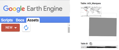
Once you press run the Console tab will show you how many scenes are available in your AOI for a given timeframe. In the tasks tab you can press run to start downloading the satellite images (as GeoTIFF files) and their dates in your Google Drive folder.
The AVOCADO algorithm does not require any pre-processing (besides the steps in GEE), but the dates of the raster stack in a certain format. The dates file is separate from the raster stack in GEE and needs to be converted to the following format: e.g. “1990-02-16” (these are needed to for all the analysis from step 3 onwards).
Step 3: Load the raster stack in R and create the reference phenological curve
|
# Loading raster dataset |
Create the vegetation reference curve (in case of forest monitoring, this should be an area of undisturbed forest such as forest in a national parc – often verified on high resolution images such as available via Google Earth Pro). It is in practice possible to create a reference based on one pixel, but it is recommended to use several pixels (think in the range of 100 - 100,000 pixels) to account for natural variation between tree species. Also when monitoring a mono specific forest stand, it is still good to include multiple pixels to account for any phenological variation that might be present within the forest stand.
For this step you need the raster stack and the reference curve. If the site location is in the northern hemisphere use h = 1 (all reference curves that look gaussian shaped or have little variation) , or h = 2 in the southern hemisphere (all reference curves that have a U-shape). This also depend on the phenological cycle of the study area.
|
# Load the dates |
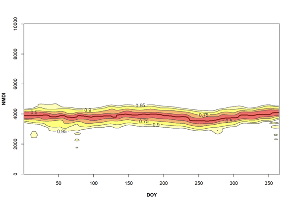
Forest reference curve for the example data
The above steps are the same for both the individual pixel level and wall-to-wall output of the algorithm. Below first the pixel level procedure and after the wall-to-wall procedure will be explained.
Step 4: Calculate the anomalies and and their likelihoods - for individual pixels
Here you will use the reference forest curve created in the previous step. It is very important to change anop = c(1:N) with n = number of layers in your SpatRaster. Every value in your time-series will be plotted against the reference and the anomaly and coinciding likelihood will be calculated.
Now we can map our anomalies (first half of the bands/layers)
|
crs.data <- crs(MDD) |
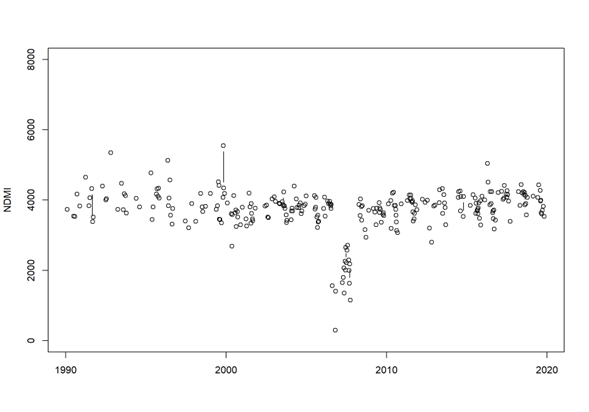 Pixel time series
|
# Anomaly calculation |
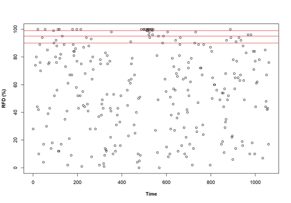
Anomaly detection and likelihoods for all the NDMI values for the pixel of interest. The red lines are 90%, 95% and 99% RFD thresholds
Step 5 Disturbance and regrowth detection - for individual pixels
Based on the anomalies and the likelihoods (rfd values), the change detection can be done. Change the parameters rfd = freq distribution; rgrow_thr = number of days that a disturbance has to stay a disturbance; dstrb_thr = number of days that regrowth has to stay regrown e.g. to avoid crops being detected as regrowth. Also the cdates (i.e. the number of consecutive observations that are below a certain threshold) can be adjusted. Please read the paper (Decuyper et al., 2022), or visit please visit Github MDecuy for more details.
|
dist.reg(x = anom_rfd, dates = MDD_dates, rfd = 0.95, dstrb_thr = 1, rgrow_thr = 730, cdates = 3) |
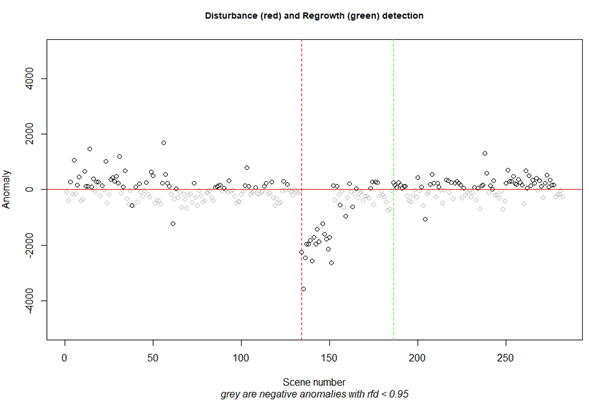
The change detection result of the pixel of interest. In the console you will find all change years (if any). In this case there was a disturbance in 2006 (red line) and a recovery in 2011 (green line)
Step 6 Calculate the anomalies and and their likelihoods – wall-to-wall output
This step will take most of the processing time so please check the computing capacity of your computer. This does not apply for the example dataset in this tutorial. The arguments are the same as for the individual pixels, but here you write your output.
|
PLUGPhenAnoRFDMapPLUS(s = MDD, dates = MDD_dates, h = 1, phenref = MDD_fref, anop = c(1:1063), nCluster = 1, outname = 'YourDirectory/MDD_AnomalyLikelihood.tif',datatype = 'INT2S') |
The output file contains all the anomalies, followed by all likelihoods and thus has twice the number of layers as the input SpatRaster.
Step 7 Disturbance and regrowth detection – wall-to-wall output
|
# 3 Load anomaly and likelihoods data ## Disturbance computation |
Also here the arguments are the same as for the individual pixels, but here you write your output. Please read the paper (Decuyper et al., 2022), or visit please visit Github MDecuy for more details.
The output file of the wall-to-wall map will always contain 16 bands as shown in the figure below (Band 1: First disturbance year; Band 2: Anomalies coinciding with the first disturbance; Band 3: First regrowth year; Band 4: Anomalies coinciding with the first regrowth; Band 5: Second disturbance year; Etc.). For example: If a pixel has only values in the first 4 bands, followed by NA’s in the next bands, the pixel had only one disturbance and one regrowth event.
Change detection output for the example data
If you use this tutorial and/or the AVOCADO algorithm, please cite:
Decuyper, Mathieu, Roberto O Chávez, Madelon Lohbeck, José A Lastra, Nandika Tsendbazar, Julia Hackländer, Martin Herold, and Tor-G Vågen. “Continuous Monitoring of Forest Change Dynamics with Satellite Time Series.” Remote Sensing of Environment 269 (2022): 112829. https://doi.org/10.1016/j.rse.2021.112829.
References
Decuyper, Mathieu, Roberto O Chávez, Madelon Lohbeck, José A Lastra, Nandika Tsendbazar, Julia Hackländer, Martin Herold, and Tor-G Vågen. “Continuous Monitoring of Forest Change Dynamics with Satellite Time Series.” Remote Sensing of Environment 269 (2022): 112829. https://doi.org/10.1016/j.rse.2021.112829.
Chávez, Roberto O., Sergio A. Estay, José A. Lastra, Carlos G. Riquelme, Matías Olea, Javiera Aguayo, and Mathieu Decuyper. “Npphen: An R-Package for Detecting and Mapping Extreme Vegetation Anomalies Based on Remotely Sensed Phenological Variability.” Remote Sensing 15, no. 1 (December 23, 2022): 73. https://doi.org/10.3390/rs15010073.
Gorelick, Noel, Matt Hancher, Mike Dixon, Simon Ilyushchenko, David Thau, and Rebecca Moore. “Google Earth Engine: Planetary-Scale Geospatial Analysis for Everyone.” Remote Sensing of Environment 202 (December 2017): 18–27. https://doi.org/10.1016/j.rse.2017.06.031.